Module 2, Practical 5¶

In this practical we will work with sorting algorithms.

Sorting algorithms¶

The basic principle of sorting algorithms is quite simple:

>given an input sequence (\(U\)) of (at least partially) un-sorted elements \(U=u_{1},u_{2}, ..., u_{n}\), output a new sequence \(S = s_{1}, s_{2}, ... , s_{n}\) which is a permutation of the elements in \(U\) such that \(s_{1}\leq s_{2}, ..., \leq s_{n}\).

Several sorting algorithms exist, the first one we will work with is selection sort.

Selection sort¶

Selection sort is the simplest of the sorting algorithms.

The idea of selection sort is that given \(U=u_{1},u_{2},...,u_{n}\) the algorithm loops through all the elements of \(U\), finds the minimum \(u_m\) and places it at the beginning of the sequence \(U\), swapping \(u_{1}\) with \(u_m\). At the next iteration, the algorithm continues looking for the minimum starting from \(u_2\) and so on.

If \(U\) has \(n\) elements, we need to perform the following two steps for each position \(i=0,..,n-1\) in the list:

(argmin) Find index of the minimum element in the sublist \(U[i:]\), let’s call it \(min\) (i.e. \(u_{min} = min(U[i:])\));
(swap) Swap \(u_{min}\) with \(u_i\);

A reminder on how selection sort works is shown in this picture taken from the lecture slides. Yellow cells are the minimum found at each iteration, while orange cells are those already sorted by previous iterations.

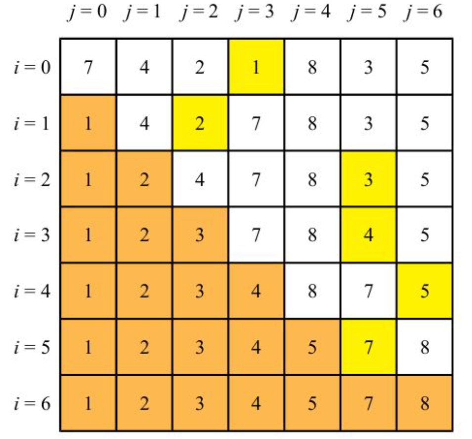
A good implementation of this sorting algorithm has complexity \(O(n^2)\), where \(n\) is the number of elements in the list to sort.

A base class for sorting algorithms¶

Implement a base class, SortingAlgorithm, that has the following attributes:

data (the actual data to sort)
operations (initialized to 0) that counts how many swaps have been done to perform the sorting
comparisons (initialized to 0) that counts how many comparisons have been done
verbose a boolean (default= True) that is used to decide if the method should report what is happening at each step and some stats or not.

The class has one method, sort, that implements the sort algorithm (empty for the base class)

[17]:

class SortingAlgorithm:
    def __init__(self, data, verbose = True):
        self.data = data
        self.comparisons = 0
        self.operations = 0
        self.verbose = verbose

    def getData(self):
        return self.data

    def getOperations(self):
        return self.operations

    def getComparisons(self):
        return self.comparisons

    def sort(self):
        raise NotImplementedError

sa = SortingAlgorithm([])
print(sa)
sa.sort()

<__main__.SortingAlgorithm object at 0x7fc80a62a940>

---------------------------------------------------------------------------
NotImplementedError                       Traceback (most recent call last)
/home/davidebrex/Documents/ESERCITAZIONI/sciprog-ds-M2-23_24/M2_practical5.ipynb Cell 4 line 2
     <a href='vscode-notebook-cell:/home/davidebrex/Documents/ESERCITAZIONI/sciprog-ds-M2-23_24/M2_practical5.ipynb#W3sZmlsZQ%3D%3D?line=19'>20</a> sa = SortingAlgorithm([])
     <a href='vscode-notebook-cell:/home/davidebrex/Documents/ESERCITAZIONI/sciprog-ds-M2-23_24/M2_practical5.ipynb#W3sZmlsZQ%3D%3D?line=20'>21</a> print(sa)
---> <a href='vscode-notebook-cell:/home/davidebrex/Documents/ESERCITAZIONI/sciprog-ds-M2-23_24/M2_practical5.ipynb#W3sZmlsZQ%3D%3D?line=21'>22</a> sa.sort()

/home/davidebrex/Documents/ESERCITAZIONI/sciprog-ds-M2-23_24/M2_practical5.ipynb Cell 4 line 1
     <a href='vscode-notebook-cell:/home/davidebrex/Documents/ESERCITAZIONI/sciprog-ds-M2-23_24/M2_practical5.ipynb#W3sZmlsZQ%3D%3D?line=16'>17</a> def sort(self):
---> <a href='vscode-notebook-cell:/home/davidebrex/Documents/ESERCITAZIONI/sciprog-ds-M2-23_24/M2_practical5.ipynb#W3sZmlsZQ%3D%3D?line=17'>18</a>     raise NotImplementedError

NotImplementedError:

Please, note that the method sort raises an exception NotImplementedError. Exceptions are used to detect and manage errors occurred during execution. Exceptions can be raised thorough the instruction raise and they can be captured by the construct try:

[10]:

import sys

try:
    f = open('myfile.txt')
    s = f.readline()
    i = int(s.strip())
except OSError as err:
    # code executed if an exception OSError is raised during the execution of the code in the try instruction block
    print("OS error: {0}".format(err))
except ValueError:
    # exception ValueError
    print("Could not convert data to an integer.")
except:
    # general exception
    print("Unexpected error:", sys.exc_info()[0])
    raise
else:
    # optional, collects code that has to be executed ONLY if no exceptions are raised
    f.close()

OS error: [Errno 2] No such file or directory: 'myfile.txt'

In our praticals we will not use extensively Python exceptions. For a detailed explanation on how to manage errors and exceptions in Python, we refer to the official language tutorial https://docs.python.org/3/tutorial/errors.html.

Exercise (implementation)¶

Implement a class SelectionSort that inherits from the base class, with the following attributes:

data (the actual data to sort)
operations (initialized to 0) that counts how many swaps have been done to perform the sorting
comparisons (initialized to 0) that counts how many comparisons have been done
verbose a boolean (default= True) that is used to decide if the method should report what is happening at each step and some stats or not.

The class implements the sort method, sort, that implements the selection sort algorithm (two more private methods might be needed to compute swap and argmin – see description above).

Once you implemented the class, test it with some data like:

[7, 5, 10, -11 ,3, -4, 99, 1]

Show/Hide Implementation

[11]:

import random

class SortingAlgorithm:
    def __init__(self, data, verbose = True):
        self.data = data
        self.comparisons = 0
        self.operations = 0
        self.verbose = verbose

    def getData(self):
        return self.data

    def getOperations(self):
        return self.operations

    def getComparisons(self):
        return self.comparisons

    def sort(self):
        raise NotImplementedError

class SelectionSort(SortingAlgorithm):

    def __swap(self, i, j):
        """
        swaps elements i and j in data.
        """
        if(i != j): #no point in swapping if i==j
            if self.verbose:
                print("Swapping position {} with {}".format(i,j))
            self.operations += 1
            tmp = self.data[i]
            self.data[i] = self.data[j]
            self.data[j] = tmp

    def __argmin(self, i):
        """
        returns the index of the smallest element of
        self.__data[i:]
        """
        mpos = i
        N = len(self.data)
        minV = self.data[mpos]
        for j in range(i + 1, N):
            if self.data[j] < minV:
                mpos = j
                minV = self.data[j]
            # keep track of what was done
            self.comparisons += 1

        return mpos

    def sort(self):
        self.comparisons = 0
        self.operations = 0

        for i in range(len(self.data) - 1):
                j = self.__argmin(i)
                self.__swap(i, j)


if __name__ == "__main__":
    # this code is executed when SelectionSort is directly executed...
    # https://docs.python.org/3/library/__main__.html
    d = [7, 5, 10, -11 ,3, -4, 99, 1]
    selSorter = SelectionSort(d, verbose = True)
    selSorter.sort()
    print(d)
    d = []

    for i in range(0,1000):
        d.append(random.randint(0,1000))
    selSorter = SelectionSort(d, verbose = False)
    selSorter.sort()
    print("\nNumber of elements: {}".format(len(d)))
    print("Number of comparisons: {}".format(selSorter.getComparisons()))
    print("Number of swaps: {}".format(selSorter.getOperations()))

    d = []
    for i in range(0,2000):
        d.append(random.randint(0,1000))
    selSorter = SelectionSort(d, verbose = False)
    selSorter.sort()
    print("\nNumber of elements: {}".format(len(d)))
    print("Number of comparisons: {}".format(selSorter.getComparisons()))
    print("Number of swaps: {}".format(selSorter.getOperations()))

    test = True
    for el in range(0,len(d)-1):
        test = test and (d[el]<= d[el+1])
    print("\nSorting test passed? {}".format(test))

Swapping position 0 with 3
Swapping position 1 with 5
Swapping position 2 with 7
Swapping position 3 with 4
Swapping position 4 with 5
Swapping position 6 with 7
[-11, -4, 1, 3, 5, 7, 10, 99]

Number of elements: 1000
Number of comparisons: 499500
Number of swaps: 990

Number of elements: 2000
Number of comparisons: 1999000
Number of swaps: 1985

Sorting test passed? True

Download the complete source file: SelectionSort.py

Insertion sort¶

The second sorting algorithm we will see is insertion sort. As for selection sort, this algorithm builds the solution one element at a time. It is not a very efficient sorting algorithm but it is quite simple and has several advantages.

Indeed, it is an in place algorithm (i.e. it does not need to copy the array to sort it therefore it is easy on memory), and it can be efficient for nearly sorted lists. This is the algorithm that people use when sorting a deck of cards.

The algorithm builds a sorted list step by step. At each iteration it removes one element from the list, placing it in the correct position within the growing sorted list.

The algorithm makes use of two indexes: \(i\) moving on the un-sorted part of the list and \(j\), on the growing sorted part of the list. The index \(i\) starts from 1 and loops up to the end of the list, while \(j\) starts from \(i\) at each iteration and goes down to finding the place where the element at index \(i\) should go in the sorted list, pushing the other elements up while finding the right place.

An element at position \(h\) is pushed-up by copying \(u_h\) to position \(h+1\).

Given an unsorted list \(U = u_0, u_1, ..., u_n\):

For each \(i\) from 1 to \(l = length(list)\):

get \(u_i\) and store it in a temporary variable \(temp\);
for \(j = i\),…,0 push \(u_{j-1}\) to position \(j\) until \(temp\) > \(u_{j-1}\). If \(j\) exists such that \(temp\) < \(u_j\), place \(temp\) at position \(j\), otherwise place \(temp\) in position \(0\).

A graphical representation of the algorithm (from the lecture slides) follows:

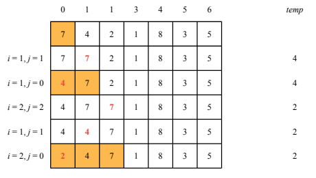
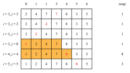
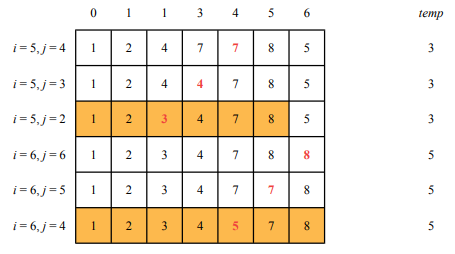
The worst case complexity of this algorithm is \(O(n^2)\), with \(n\) being the number of elements in the list. If one element is no more than \(k\) places away from its place in the sorted array, the real complexity goes to \(O(kn)\). The cost of the algorithm is therefore dependent on the sorting of the input list.

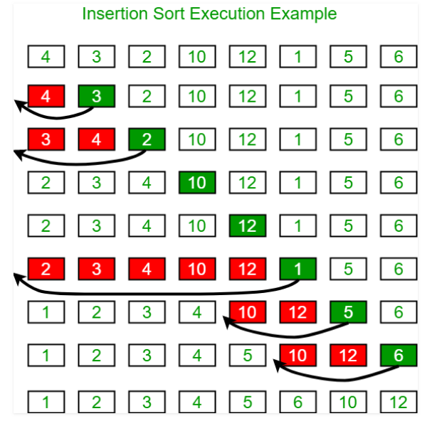
Another graphical representation of the algorithm follows (from geeksforgeeks.org). At each iteration, red boxes are pushed to the right to make room for the green element.

Exercise (implementation)¶

Implement a class InsertionSort that inherits from the base class and has the following attributes:

data (the actual data to sort)
operations (initialized to 0) that counts how many swaps (movements of data to the left) have been done to perform the sorting
comparisons (initialized to 0) that counts how many comparisons have been done
verbose, a boolean (default= True) used to decide if the method should report what is happening at each step and some stats or not

The class should implement the sort method.

Show/Hide Implementation

[12]:

import random

class SortingAlgorithm:
    def __init__(self, data, verbose = True):
        self.data = data
        self.comparisons = 0
        self.operations = 0
        self.verbose = verbose

    def getData(self):
        return self.data

    def getOperations(self):
        return self.operations

    def getComparisons(self):
        return self.comparisons

    def sort(self):
        raise NotImplementedError

class InsertionSort(SortingAlgorithm):

    def sort(self):
        self.comparisons = 0
        self.operations = 0

        for i in range(1, len(self.data)):
            temp = self.data[i]
            j = i
            while j > 0 and self.data[j-1] > temp:
                self.data[j] = self.data[j - 1]
                self.operations += 1
                self.comparisons += 1
                j = j - 1

            self.data[j] = temp
            self.operations += 1
            if j > 0:
                self.comparisons += 1
            if self.verbose:
                print("It. {}: {} comp: {} push+place:{}".format(i,
                                                           self.data,
                                                           self.comparisons,
                                                           self.operations
                                                          ))

        if self.verbose:
            print(self.data)
            print("\nNumber of comparisons: {}".format(self.comparisons))
            print("Number of push-ups+place: {}".format(self.operations))


if __name__ == "__main__":
    # this code is executed when SelectionSort is directly executed...
    # https://docs.python.org/3/library/__main__.html
    d = [7, 5, 10, -11 ,3, -4, 99, 1]
    insSorter = InsertionSort(d, verbose = True)
    insSorter.sort()
    print(d)

    d = []
    for i in range(0,1000):
        d.append(random.randint(0,1000))
    insSorter = InsertionSort(d, verbose = False)
    insSorter.sort()
    print("\nNumber of elements: {}".format(len(d)))
    print("Number of comparisons: {}".format(insSorter.getComparisons()))
    print("Number of push-ups+place: {}".format(insSorter.getOperations()))

    d = []
    for i in range(0,2000):
        d.append(random.randint(0,1000))
    insSorter = InsertionSort(d, verbose = False)
    insSorter.sort()
    print("\nNumber of elements: {}".format(len(d)))
    print("Number of comparisons: {}".format(insSorter.getComparisons()))
    print("Number of push-ups+place: {}".format(insSorter.getOperations()))

    test = True
    for el in range(0,len(d)-1):
        test = test and (d[el]<= d[el+1])
    print("\nSorting test passed? {}".format(test))

It. 1: [5, 7, 10, -11, 3, -4, 99, 1] comp: 1 push+place:2
It. 2: [5, 7, 10, -11, 3, -4, 99, 1] comp: 2 push+place:3
It. 3: [-11, 5, 7, 10, 3, -4, 99, 1] comp: 5 push+place:7
It. 4: [-11, 3, 5, 7, 10, -4, 99, 1] comp: 9 push+place:11
It. 5: [-11, -4, 3, 5, 7, 10, 99, 1] comp: 14 push+place:16
It. 6: [-11, -4, 3, 5, 7, 10, 99, 1] comp: 15 push+place:17
It. 7: [-11, -4, 1, 3, 5, 7, 10, 99] comp: 21 push+place:23
[-11, -4, 1, 3, 5, 7, 10, 99]

Number of comparisons: 21
Number of push-ups+place: 23
[-11, -4, 1, 3, 5, 7, 10, 99]

Number of elements: 1000
Number of comparisons: 245791
Number of push-ups+place: 245797

Number of elements: 2000
Number of comparisons: 983021
Number of push-ups+place: 983029

Sorting test passed? True

Download the complete source file: InsertionSort.py

Merge sort and Quick sort¶

These are divide et impera algorithms (latin, divide and conquer in English) and they work by:

dividing the original problem in smaller problems (based on parameters such as the size of the input list);
recursively solving the smaller problems (splitting them until the minimum unit – the base case – is reached and solved);
combining the partial results in the final solution.

Merge sort¶

The idea of merge sort is that given an unsorted list \(U=u_{1},u_{2},...,u_{n}\) the \(MergeSort\) procedure:

breaks the list \(U\) in two similarly sized lists (if the size is odd, the first list is always one element bigger than the other);
calls \(MergeSort\) recursively on the two sublists, until we have sublists of one element only, which are ordered by definition;
merges the two already sorted sublists in a sorted list.

The base-case of this algorithm is that lists with size \(0\) or \(1\) are ordered and are ready to be merged, therefore the algorithm keeps splitting partial lists in two sublists until these reach the length \(0\) or \(1\). At that point the two lists are merged into a bigger sorted list by using a merge method.

This is done recursively until only one list is obtained, which is the final result.

The algorithm makes use of three methods:

(merge): gets two sorted lists and produces a sorted list that contains all the elements of the two lists. This method builds the return list by getting the minimum element of the two lists, “removing” it from the corresponding list and appending it to the list with the result. “removal” can be done by using two indexes pointing to the smallest elements of each of the two (sub)lists and incrementing the index of the minimum of the two (i.e. the element that is also copied to the result list);
(recursiveMergeSort): gets an unordered (sub)list, the index of the beginning of the list, and the index of the end of the list. It recursively splits it in two halves until it reaches lists with length \(0\) or \(1\) - at that point it starts merging pairs of sorted lists to build the result;
(mergeSort) gets a list and applies the recursiveMergeSort method to it starting from position \(0\) to \(len - 1\).

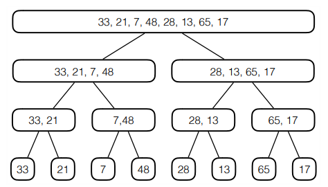
A reminder on how merge sort works is shown here (from the lecture slides). The first part is the splitting of the initial list into smaller lists, until the base level is reached with recursiveMergeSort.

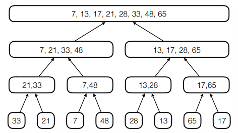
This second picture shows how the sorted list can be reconstructed by applying the merge method to pairs of sorted lists.

A good implementation of this sorting algorithm has complexity \(O(n log (n))\) where \(n\) is the number of elements in the list to sort.

Exercise (Implementation)¶

Implement a class MergeSort that inherits from the base class and has the following attributes:

data (the actual data to sort)
operations (initialized to 0) that counts how many recursive calls have been done to perform the sorting
comparisons (initialized to 0) that counts how many comparisons have been done
time attribute that keeps track of the elapsed time (hint: use the Python time module)
verbose a boolean (default= True) that is used to decide if the method should report what is happening at each step and some stats or not.

The class implements the sort method that implements the merge sort algorithm (two more private methods might be needed to compute merge and recursiveMergeSort – see description above).

Once you implemented the class you can test it with some data like:

[7, 5, 10, -11 ,3, -4, 99, 1]

Show/Hide Implementation

[13]:

import random
import time

class SortingAlgorithm:
    def __init__(self, data, verbose = True):
        self.data = data
        self.comparisons = 0
        self.operations = 0
        self.verbose = verbose

    def getData(self):
        return self.data

    def getOperations(self):
        return self.operations

    def getComparisons(self):
        return self.comparisons

    def sort(self):
        raise NotImplementedError

class MergeSort(SortingAlgorithm):
    def __init__(self,data, verbose = True):
        self.data = data
        self.time = 0
        self.comparisons = 0
        self.operations = 0
        self.verbose = verbose

    def getTime(self):
        return(self.time)

    def __merge(self, first, last, mid):
        if self.verbose:
            print("Executing merge({},{},{})...".format(first,last,mid))
        tmp = []
        i = first
        j = mid + 1
        while i <= mid and j <= last:
            if self.data[i] < self.data[j]:
                tmp.append(self.data[i])
                i += 1
            else:
                tmp.append(self.data[j])
                j += 1
            self.comparisons += 1
        while i <= mid:
            tmp.append(self.data[i])
            i += 1
        self.data[first:first+len(tmp)] = tmp

    def __recursiveMergeSort(self, first, last):
        if self.verbose:
            print("Executing recursive merge sort({},{})...".format(first,last))

        self.operations += 1
        if first < last:
            mid = (first + last)//2 #<- index so mid+1 elements go in the first sublist!!!
            self.__recursiveMergeSort(first, mid)
            self.__recursiveMergeSort(mid +1, last)
            self.__merge(first,last,mid)

    def sort(self):
        self.comparisons = 0
        self.operations = 0
        start = time.time()
        self.__recursiveMergeSort(0,len(self.data)-1)
        end = time.time()
        self.time = end - start



if __name__ == "__main__":
    # this code is executed when SelectionSort is directly executed...
    # https://docs.python.org/3/library/__main__.html
    d = [7, 5, 10, -11 ,3, -4, 99]
    mergeSorter = MergeSort(d, verbose = True)
    mergeSorter.sort()
    print(d)

    d = []
    for i in range(0,1000):
        d.append(random.randint(0,1000))
    mergeSorter = MergeSort(d, verbose = False)
    mergeSorter.sort()
    print("\nNumber of elements: {}".format(len(d)))
    print("Number of comparisons: {}".format(mergeSorter.getComparisons()))
    print("Number of swaps: {}".format(mergeSorter.getOperations()))
    print("In {:.4f}s".format(mergeSorter.getTime()))

    d = []
    for i in range(0,2000):
        d.append(random.randint(0,1000))
    mergeSorter = MergeSort(d, verbose = False)
    mergeSorter.sort()
    print("\nNumber of elements: {}".format(len(d)))
    print("Number of comparisons: {}".format(mergeSorter.getComparisons()))
    print("Number of recursions: {}".format(mergeSorter.getOperations()))
    print("In {:.4f}s".format(mergeSorter.getTime()))

    test = True
    for el in range(0,len(d)-1):
        test = test and (d[el]<= d[el+1])
    print("\nSorting test passed? {}".format(test))

Executing recursive merge sort(0,6)...
Executing recursive merge sort(0,3)...
Executing recursive merge sort(0,1)...
Executing recursive merge sort(0,0)...
Executing recursive merge sort(1,1)...
Executing merge(0,1,0)...
Executing recursive merge sort(2,3)...
Executing recursive merge sort(2,2)...
Executing recursive merge sort(3,3)...
Executing merge(2,3,2)...
Executing merge(0,3,1)...
Executing recursive merge sort(4,6)...
Executing recursive merge sort(4,5)...
Executing recursive merge sort(4,4)...
Executing recursive merge sort(5,5)...
Executing merge(4,5,4)...
Executing recursive merge sort(6,6)...
Executing merge(4,6,5)...
Executing merge(0,6,3)...
[-11, -4, 3, 5, 7, 10, 99]

Number of elements: 1000
Number of comparisons: 8713
Number of swaps: 1999
In 0.0022s

Number of elements: 2000
Number of comparisons: 19409
Number of recursions: 3999
In 0.0047s

Sorting test passed? True

Download the complete source file: MergeSort.py

Quick sort¶

The last sorting algorithm we will see is quick sort. As for merge sort, this algorithm follows the divide et impera paradigm and its easiest implementation is recursive.

The idea is that, given an unsorted list \(U = u_1, ..., u_n\), at each step a pivot \(j\) is selected and elements are rearranged in a way that all \(u_i\) such that \(u_i < u_j\) are placed at the left of \(u_j\) and all \(u_h\) such that \(u_h\) > \(u_j\) are placed to the right of \(u_j\).

This divide and conquer approach works like that:

(divide) partition the initial list \(U = u_1, .., u_n\) in two non-empty sublists (reordering the elements) such that all the elements in the first sublist are lower than the elements in the second. The pivot element \(u_j\) is such that all the elements \(u_i\) for \(1 \leq i \lt j\) are lower than \(u_j\) and all \(u_k\) for \(k > j\) are higher than \(u_j\);
(conquer) each sublist is recurisvely partitioned in two sublists, repeating until single elements are reached;
(recombine) nothing is left to do to recombine the results.

A graphical representation of the algorithm follows (red elements are the pivot of each sublist):

The algorithm makes use of the following methods:

pivot: gets the list, a start and end index, sets the first element as pivot and reorders all the elements in the list from start to end in such a way that all the elements to the left of the pivot (i.e. having index lower) are smaller than the pivot and all the elements to the right (i.e. with index higher) are bigger than the pivot. The function returns the index of the pivot;
swap: gets two indexes and swaps their values;
recursiveQuickSort: gets an unordered (sub)list, with start and end positions and finds the pivot and recursively applies the same procedure to the sublists to the left and right of the pivot;
quickSort: gets an unordered list and applies the recursive quick sort procedure to it.

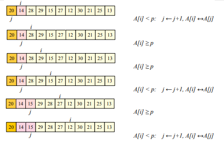
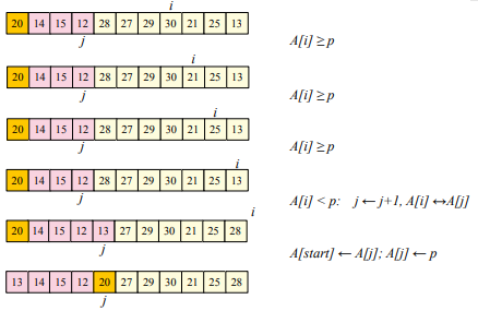
The pivot method is shown below (from lecture slides). The pivot is initially set to the first element of the sublist, then all the elements in the interval start - end are compared to it (using an index \(i\)) and placed right after the pivot if smaller (updating an index \(j\) on where the pivot should go at the end of the procedure), left untouched otherwise. At the end the pivot is moved to position \(j\). The pivot is yellow and moved elements are pink:

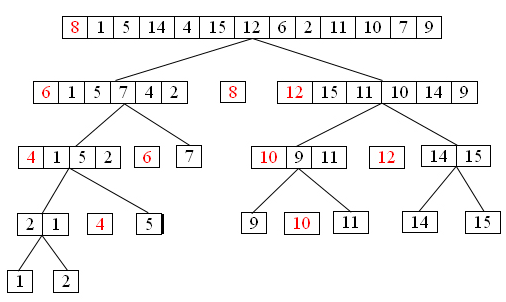
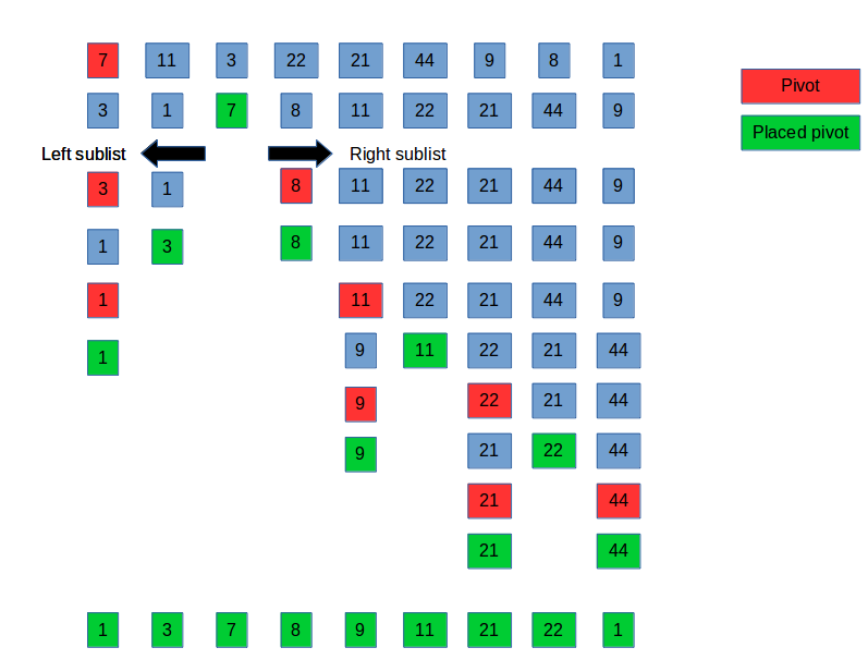
Another graphical representation follows. This picture highlights the selection of pivots (red), their placing after the (pivot) method (green) and the split of the two sublists in correspondence of the placed pivot.

The average case complexity of the quick sort algorithm is \(O(n log n)\) with \(n\) being the number of elements in the list. The worst case complexity is \(O(n^2)\) which is worse than merge sort’s \(O(n log n)\). In general, however, it performs better than merge sort.

Exercise (Implementation)¶

Implement a class QuickSort that inherits from the base class and has the following attributes:

data (the actual data to sort)
operations (initialized to 0) that counts how many swaps (movements of data to the left) have been done to perform the sorting
comparisons (initialized to 0) that counts how many comparisons have been done
verbose a boolean (default= True) that is used to decide if the method should report what is happening at each step and some stats or not.

The class implements the method called sort that implements the quick sort algorithm (which will use the private methods pivot, swap and recQuickSort– see description above).

How long does it take with a list of 10,000 elements? With 300,000?

Show/Hide Implementation

[14]:

import random
import time

class SortingAlgorithm:
    def __init__(self, data, verbose = True):
        self.data = data
        self.comparisons = 0
        self.operations = 0
        self.verbose = verbose

    def getData(self):
        return self.data

    def getOperations(self):
        return self.operations

    def getComparisons(self):
        return self.comparisons

    def sort(self):
        raise NotImplementedError

class QuickSort(SortingAlgorithm):
    def __init__(self,data, verbose = True):
        self.data = data
        self.time = 0
        self.comparisons = 0
        self.operations = 0
        self.verbose = verbose

    def getTime(self):
        return(self.time)

    def __swap(self, i,j):
        """swaps elements at positions i and j"""
        if(i != j): # no point in swapping if i==j
            self.operations += 1
            tmp = self.data[i]
            self.data[i] = self.data[j]
            self.data[j] = tmp

    def __pivot(self, start, end):
        """gets the pivot and swaps elements in [start, end]
        accordingly"""
        p = self.data[start]
        j = start

        for i in range(start + 1, end + 1):
            self.comparisons += 1
            if self.data[i] < p:
                j = j + 1
                self.__swap(i, j)

        self.__swap(start,j)

        return j

    def __recQuickSort(self, start, end):
        """gets the pivot and recursively applies
        itself on the left and right sublists
        """
        if start < end:
            #GET THE PIVOT
            j = self.__pivot(start, end)

            self.__recQuickSort(start, j - 1)

            self.__recQuickSort(j + 1, end)

    def sort(self):
        self.comparisons = 0
        self.operations = 0
        start = time.time()
        self.__recQuickSort(0, len(self.data) - 1)
        end = time.time()
        self.time = end - start


if __name__ == "__main__":
    # this code is executed when SelectionSort is directly executed...
    # https://docs.python.org/3/library/__main__.html
    d = [7, 3, 10, -11 ,5, -4, 99, 1]
    qkSorter = QuickSort(d, verbose = True)
    qkSorter.sort()
    d = []

    for i in range(0,1000):
        d.append(random.randint(0,1000))
    qkSorter = QuickSort(d, verbose = False)
    qkSorter.sort()
    print("\nNumber of elements: {}".format(len(d)))
    print("Number of comparisons: {}".format(qkSorter.getComparisons()))
    print("Number of push-ups+place: {}".format(qkSorter.getOperations()))
    print("In {:.4f}s".format(qkSorter.getTime()))

    d = []
    for i in range(0,10000):
        d.append(random.randint(0,1000))
    qkSorter = QuickSort(d, verbose = False)
    qkSorter.sort()
    print("\nNumber of elements: {}".format(len(d)))
    print("Number of comparisons: {}".format(qkSorter.getComparisons()))
    print("Number of push-ups+place: {}".format(qkSorter.getOperations()))
    print("In {:.4f}s".format(qkSorter.getTime()))
    test = True

    d = []
    for i in range(0,300000):
        d.append(random.randint(0,1000))
    qkSorter = QuickSort(d, verbose = False)
    qkSorter.sort()
    print("\nNumber of elements: {}".format(len(d)))
    print("Number of comparisons: {}".format(qkSorter.getComparisons()))
    print("Number of push-ups+place: {}".format(qkSorter.getOperations()))
    print("In {:.4f}s".format(qkSorter.getTime()))
    test = True

    for el in range(0,len(d)-1):
        test = test and (d[el]<= d[el+1])
    print("\nSorting test passed? {}".format(test))


Number of elements: 1000
Number of comparisons: 11367
Number of push-ups+place: 5405
In 0.0024s

Number of elements: 10000
Number of comparisons: 175503
Number of push-ups+place: 58458
In 0.0317s

Number of elements: 300000
Number of comparisons: 48681219
Number of push-ups+place: 1873741
In 4.5578s

Sorting test passed? True

Download the complete source file: QuickSort.py

Exercise (algorithm benchmark)¶

Write some python code to test the performance of selection sort, insertion sort, merge sort and quick sort with different lists of incremental size. Test the algorithms, reporting stats and running time.

To complete the exercise, you will need to add the time measurement feature to the base SortingAlgorithm class and modify all four child classes accordingly.

Finally, challenge them with the following arrays:

list(range(5000))
c = list(range(5000)); c.sort(reverse=True) (reverse-sorted, worst case scenario)
a = list(range(1000)); b = list(range(1000,2000)); b.sort(reverse=True); sort(a+b)

Show/Hide Solution

[15]:

import random
import sys
import time

class SortingAlgorithm:
    def __init__(self, data, verbose = True):
        self.data = data
        self.comparisons = 0
        self.operations = 0
        self.time = 0 # novel addition!
        self.verbose = verbose

    def getData(self):
        return self.data

    def getOperations(self):
        return self.operations

    def getComparisons(self):
        return self.comparisons

    def getTime(self):
        return(self.time) # novel addition!

    def sort(self):
        raise NotImplementedError


class SelectionSort(SortingAlgorithm):

    def __swap(self, i, j):
        """
        swaps elements i and j in data.
        """
        if(i != j): #no point in swapping if i==j
            if self.verbose:
                print("Swapping position {} with {}".format(i,j))
            self.operations += 1
            tmp = self.data[i]
            self.data[i] = self.data[j]
            self.data[j] = tmp

    def __argmin(self, i):
        """
        returns the index of the smallest element of
        self.__data[i:]
        """
        mpos = i
        N = len(self.data)
        minV = self.data[mpos]
        for j in range(i + 1, N):
            if self.data[j] < minV:
                mpos = j
                minV = self.data[j]
            # keep track of what was done
            self.comparisons += 1

        return mpos

    def sort(self):
        start = time.time()
        self.comparisons = 0
        self.operations = 0

        for i in range(len(self.data) - 1):
                j = self.__argmin(i)
                self.__swap(i, j)
                # keep track of what was done
                self.operations += 1

        end = time.time()
        self.time = end - start

class InsertionSort(SortingAlgorithm):

    def sort(self):
        start = time.time()
        self.comparisons = 0
        self.operations = 0

        for i in range(1, len(self.data)):
            temp = self.data[i]
            j = i
            while j > 0 and self.data[j-1] > temp:
                self.data[j] = self.data[j - 1]
                self.operations += 1
                self.comparisons += 1
                j = j - 1

            self.data[j] = temp
            self.operations += 1
            if j > 0:
                self.comparisons += 1
            if self.verbose:
                print("It. {}: {} comp: {} push+place:{}".format(i,
                                                           self.data,
                                                           self.comparisons,
                                                           self.operations
                                                          ))

        if self.verbose:
            print(self.data)
            print("\nNumber of comparisons: {}".format(self.comparisons))
            print("Number of push-ups+place: {}".format(self.operations))

        end = time.time()
        self.time = end - start


class MergeSort(SortingAlgorithm):
    def __init__(self,data, verbose = True):
        self.data = data
        self.time = 0
        self.comparisons = 0
        self.operations = 0
        self.verbose = verbose

    def __merge(self, first, last, mid):
        if self.verbose:
            print("Executing merge({},{},{})...".format(first,last,mid))
        tmp = []
        i = first
        j = mid + 1
        while i <= mid and j <= last:
            if self.data[i] < self.data[j]:
                self.comparisons += 1
                tmp.append(self.data[i])
                i += 1
            else:
                tmp.append(self.data[j])
                j += 1
        while i <= mid:
            tmp.append(self.data[i])
            i += 1
        self.data[first:first+len(tmp)] = tmp

    def __recursiveMergeSort(self, first, last):
        if self.verbose:
            print("Executing recursive merge sort({},{})...".format(first,last))

        self.operations += 1
        if first < last:
            mid = (first + last)//2 #<- index so mid+1 elements go in the first sublist!!!
            self.__recursiveMergeSort(first, mid)
            self.__recursiveMergeSort(mid +1, last)
            self.__merge(first,last,mid)

    def sort(self):
        self.comparisons = 0
        self.operations = 0
        start = time.time()
        self.__recursiveMergeSort(0,len(self.data)-1)
        end = time.time()
        self.time = end - start

class QuickSort(SortingAlgorithm):
    def __init__(self,data, verbose = True):
        self.data = data
        self.time = 0
        self.comparisons = 0
        self.operations = 0
        self.verbose = verbose

    def __swap(self, i,j):
        """swaps elements at positions i and j"""
        self.operations += 1
        tmp = self.data[i]
        self.data[i] = self.data[j]
        self.data[j] = tmp

    def __pivot(self, start, end):
        """gets the pivot and swaps elements in [start, end]
        accordingly"""
        p = self.data[start]
        j = start

        for i in range(start + 1, end + 1):
            self.comparisons += 1
            if self.data[i] < p:
                j = j + 1
                self.__swap(i, j)

        self.__swap(start,j)

        return j

    def __recQuickSort(self, start, end):
        """gets the pivot and recursively applies
        itself on the left and right sublists
        """
        if start < end:
            #GET THE PIVOT
            j = self.__pivot(start, end)

            self.__recQuickSort(start, j - 1)

            self.__recQuickSort(j + 1, end)

    def sort(self):
        self.comparisons = 0
        self.operations = 0
        start = time.time()
        self.__recQuickSort(0, len(self.data) - 1)
        end = time.time()
        self.time = end - start


#Need to extend the recursion limit for the test on reverse sorted
#array with 5000 elements
sys.setrecursionlimit(10000)
def getNrandom(n):
    res = []
    for i in range(n):
        res.append(random.randint(-10000,10000))
    return res

def testSorters(myList, verbose = False):
    #copy because the sorter will actually change the list!
    myList1 = myList[:]
    myList2 = myList[:]
    myList3 = myList[:]
    selSorter = SelectionSort(myList, verbose = False)
    insSorter = InsertionSort(myList1, verbose = False)
    mSorter = MergeSort(myList2, verbose = False)
    qSorter = QuickSort(myList3, verbose = False)
    if verbose:
        print("TestList:\n{}".format(myList))
        print("TestList1:\n{}".format(myList1))
        print("TestList2:\n{}".format(myList2))
        print("TestList3:\n{}".format(myList3))
    selSorter.sort()
    insSorter.sort()
    mSorter.sort()
    qSorter.sort()
    if verbose:
        print("Outputs:")
        print(myList)
        print(myList1)
        print(myList2)
        print(myList3)
    print("Test with {} elements".format(len(myList)))
    print("Insertion sort:")
    print("Number of comparisons: {}".format(insSorter.getComparisons()))
    print("Number of operations: {}".format(insSorter.getOperations()))
    print("In {:.4f}s".format(insSorter.getTime()))
    print("Selection sort:")
    print("Number of comparisons: {}".format(selSorter.getComparisons()))
    print("Number of operations: {}".format(selSorter.getOperations()))
    print("In {:.4f}s".format(selSorter.getTime()))
    print("Merge sort:")
    print("Number of comparisons: {}".format(mSorter.getComparisons()))
    print("Number of operations: {}".format(mSorter.getOperations()))
    print("In {:.4f}s".format(mSorter.getTime()))
    print("Quick sort:")
    print("Number of comparisons: {}".format(qSorter.getComparisons()))
    print("Number of operations: {}".format(qSorter.getOperations()))
    print("In {:.4f}s".format(qSorter.getTime()))

# script that finally executes the comparisons...
print("Test with a list of 10 elements...")
testList = getNrandom(10)
testSorters(testList, verbose = True) # just for testing that everything is OK...
print("#############")
print("Test with a list of 5000 elements...")
testList = list(range(5000))
testSorters(testList, verbose = False)
print("#############")
print("Test with a list of 5000 elements in reverse order...")
testList = list(range(5000))
testList.sort(reverse = True)
testSorters(testList, verbose = False)
print("#############")
print("Test with a list of 2000 elements, with last half in reverse order...")
a = list(range(1000))
b = list(range(1000,2000))
b.sort(reverse=True)
testSorters(a+b, verbose = False)

Test with a list of 10 elements...
TestList:
[-1526, -2117, -2465, 8732, -9668, 5762, -3382, -5152, 4468, 7148]
TestList1:
[-1526, -2117, -2465, 8732, -9668, 5762, -3382, -5152, 4468, 7148]
TestList2:
[-1526, -2117, -2465, 8732, -9668, 5762, -3382, -5152, 4468, 7148]
TestList3:
[-1526, -2117, -2465, 8732, -9668, 5762, -3382, -5152, 4468, 7148]
Outputs:
[-9668, -5152, -3382, -2465, -2117, -1526, 4468, 5762, 7148, 8732]
[-9668, -5152, -3382, -2465, -2117, -1526, 4468, 5762, 7148, 8732]
[-9668, -5152, -3382, -2465, -2117, -1526, 4468, 5762, 7148, 8732]
[-9668, -5152, -3382, -2465, -2117, -1526, 4468, 5762, 7148, 8732]
Test with 10 elements
Insertion sort:
Number of comparisons: 28
Number of operations: 31
In 0.0000s
Selection sort:
Number of comparisons: 45
Number of operations: 17
In 0.0000s
Merge sort:
Number of comparisons: 11
Number of operations: 19
In 0.0000s
Quick sort:
Number of comparisons: 21
Number of operations: 18
In 0.0000s
#############
Test with a list of 5000 elements...
Test with 5000 elements
Insertion sort:
Number of comparisons: 4999
Number of operations: 4999
In 0.0012s
Selection sort:
Number of comparisons: 12497500
Number of operations: 4999
In 1.0421s
Merge sort:
Number of comparisons: 32004
Number of operations: 9999
In 0.0089s
Quick sort:
Number of comparisons: 12497500
Number of operations: 4999
In 1.0317s
#############
Test with a list of 5000 elements in reverse order...
Test with 5000 elements
Insertion sort:
Number of comparisons: 12497500
Number of operations: 12502499
In 2.8552s
Selection sort:
Number of comparisons: 12497500
Number of operations: 7499
In 1.1662s
Merge sort:
Number of comparisons: 0
Number of operations: 9999
In 0.0088s
Quick sort:
Number of comparisons: 12497500
Number of operations: 6254999
In 2.2319s
#############
Test with a list of 2000 elements, with last half in reverse order...
Test with 2000 elements
Insertion sort:
Number of comparisons: 501499
Number of operations: 501499
In 0.1203s
Selection sort:
Number of comparisons: 1999000
Number of operations: 2499
In 0.1722s
Merge sort:
Number of comparisons: 6044
Number of operations: 3999
In 0.0032s
Quick sort:
Number of comparisons: 1999000
Number of operations: 251999
In 0.2137s

Download the complete source file: Comparison.py

Exercise (Counting Sort)¶

Implement counting sort for a list of elements included in the range [min, max]. Counting sort’s code for the simplified case of numbers in the range [0, n] is reported below:

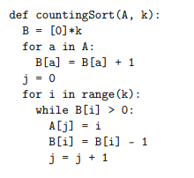
Please note that values below zero might be present too.

Show/Hide Solution